Multi-Layer Perceptron (MLP) stands as one of the pioneering architectures in deep learning neural networks (DNN). Renowned for its power and simplicity, MLPs have laid the foundation for many subsequent advancements in the field. In this article, we delve into the science behind MLPs, explore their diverse applications, and walk through the process of coding a basic classification neural network using this influential architecture.
Setup
How do humans learn? We tackle real-world problems by interpreting signals and information based on our own understanding of the world, using our brains to devise solutions. However, computers, while powerful, simply process numbers rather than raw signals efficiently (for now!). So, what exactly is meant by machine learning if computers cannot directly interpret these signals? Essentially, it involves mapping certain numerical computations to solve real-world problems. How do we achieve this? By translating real-world phenomena into numerical representations that computers can comprehend and manipulate. For instance, images are converted into pixels, essentially sets of numbers, while textual sentences are transformed into tokens, also represented by numbers.
Let’s set up a scenario: Imagine we have a real-world problem, such as image classification. We start with an input, say an image, and through cognitive processes, we identify and label what it represents. Next, we translate this human-generated understanding into a format understandable by computers. Here are the steps:
- Convert the image into numbers (input).
- Convert the output text into numbers (labels).
- Establish a relationship between them through machine learning.
The mathematical concept of functions forms the foundation of machine learning, representing relationships between sets of numbers. The set of inputs is termed the domain, while the set of outputs is called the range. Suppose, by some magic, we acquire a set of input and output pairs. It becomes apparent that predicting the exact function from these samples is impossible; the best we can do is approximate it. How? Here’s a simplified approach:
- Randomly (or through heuristics), select a family of functions (e.g., polynomial, sine, exponential).
- Identify all functions capable of mapping these input-output pairs (represented by the training data space).
- Choose the best function from this set.
Steps 1 and 2 are relatively straightforward. But how do we tackle step 3? We employ another function, an objective function, which provides a score proportional to the function’s effectiveness. This objective function, often called the loss, aims to minimize the discrepancy between predicted and actual values for a given input. Leveraging calculus, we limit ourselves to continuous functions in step 1. If the loss is also continuous, we can solve the minimization problem by computing the gradient of the loss and moving in the direction of its minimum. Learn about Gradient descent.
An important concept to grasp is that any continuous function can be approximated using polynomial functions (Taylor series approximation).
At this juncture, the setup may seem mundane, but it sets the stage for understanding how MLP fits into this framework:
- MLP is one of the families of functions (Step 1) we choose to solve a problem.
- Typically, an MLP represents a complex continuous function (involving dot producs to form another vector) with activations.
- This implies that MLP is continuous, and we can compute its gradient.
- We utilize gradients to minimize the loss, thereby identifying the best MLP parameters.
How does this MLP Look ?
The image below depicts the structure of an MLP network, but to the uninitiated eye, the jumble of lines and nodes can seem perplexing. What exactly do these elements represent?
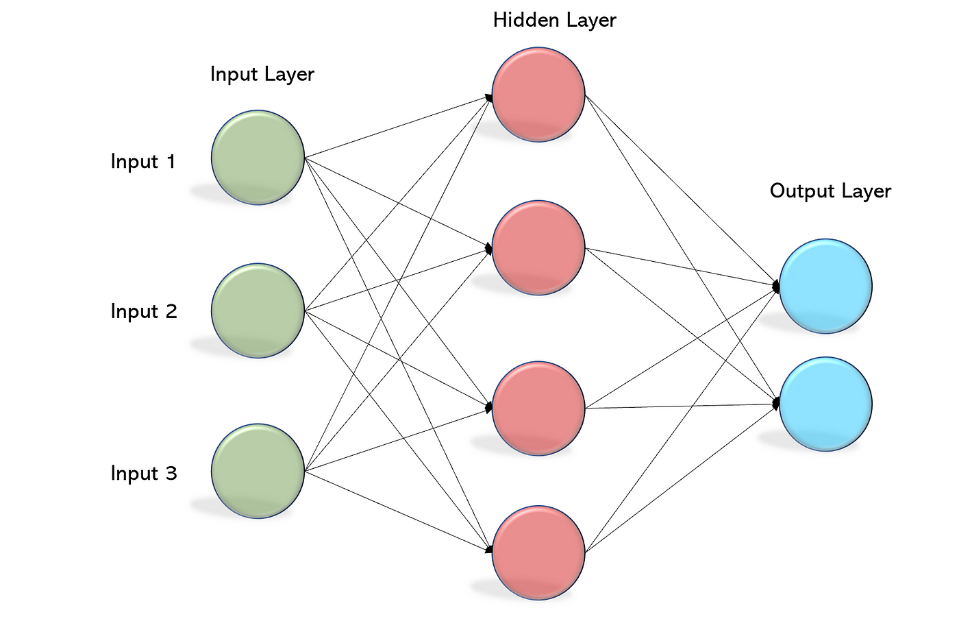
Let’s break down the components visible in the image:
- Edges: These are the lines connecting various nodes in the network.
- Neuron: Each circle or node represents a neuron in the network.
- Layers: The network comprises different layers, including input, hidden, and output layers. Now, let’s delve into the structure and concepts underlying these components.
Edges/Connections
The edges within this network symbolize numerical values, serving as representations of real-world problems that the network operates upon. These numerical representations can take various forms, but for simplicity, let’s consider them as numbers. Each node in the layerr forms a set of numbers, a vector. This vectorization facilitates efficient computation during inference.
When each neuron is connected to every other neuron in the subsequent layer, we refer to this arrangement as a fully connected layer.
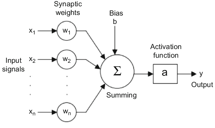
Nodes
These units are termed neurons, akin to their biological counterparts. But what exactly do they do?
Each neuron stores a numerical value for every input connection it receives. Consequently, every neuron possesses a set of these numbers, which collectively form vectors known as the neuron’s weights. One can think of these weights as reflecting the importance that each input holds for the neuron. To compute an output from the neuron, we perform a weighted sum of the input values by multiplying them with their corresponding weights and then adding them together. In essence, this operation boils down to the vector dot product between the input vector (formed by the input connections) and the weight vector.
To imbue neurons with greater expressive power, we introduce an activation operation on the output. This activation operation introduces non-linearity, expanding the repertoire of functions that the neurons can represent.
Bias
We include a bias number for each neuron because it acts as a reference point from which learning can commence. If we were to initialize all weights to zero, the network would encounter difficulties in learning. Alternatively, utilizing random initialization introduces inherent bias, providing the network with diverse starting conditions essential for effective learning.
Layer
We can observe that neurons can be grouped based on their positional similarity within the network. The layer that directly receives input numbers is termed the input layer, while the layer responsible for outputting the predicted values is referred to as the output layer. In contrast, the intermediate layers lack any direct physical interpretation. Instead, they represent mappings of intermediate functions within the numerical space. Consequently, these layers are termed hidden layers.
Why MLP is relevant ?
MLP plays the role of universal function approximator, it is because the model can represent any continuous function given enough neurons. This makes it a powerful tool.
Using pytorch to implement MLP
1. Imports
import torch
import torchvision
import torchvision.transforms as transforms
2. Defining Transforms and Loading the Dataset.
Purpose of Transform:
- Convert the raw pixels to Tensors.
- Normalize the data from -1 to 1.
transform = transforms.Compose(
    [transforms.ToTensor(),
     transforms.Normalize((0.5, 0.5, 0.5), (0.5, 0.5, 0.5))]
)

batch_size = 1

trainset = torchvision.datasets.CIFAR10(root="./data", train=True,
			download=True, transform=transform)
trainloader = torch.utils.data.DataLoader(trainset,
			batch_size=batch_size, shuffle=True, num_workers=2)

testset = torchvision.datasets.CIFAR10(root="./data", train=False,
			download=True, transform=transform)
testloader = torch.utils.data.DataLoader(testset,
			batch_size=batch_size, shuffle=False, num_workers=2)

classes = ('plane', 'car', 'bird', 'cat',
           'deer', 'dog', 'frog', 'horse', 'ship', 'truck')

print(f"shape of images: {next(iter(trainloader))[0].shape}")
print(f"shape of labels: {next(iter(trainloader))[1].shape}")
The torchvision data set gives pixel value from 0 to 1, but we create -1 to 1 (helps in utilizing relu and other advantages). The first tuple contains mean across each channel and the second tuple contains standard deviation across each channel. We then for each value normlize using this formula:
$$ \hat{x} = \dfrac{x - mean}{std} $$Doing this on values with range [0, 1] using mean=0.5 and std=0.5, results in normalized value from [-1, 1]
3. Defining our MLP architecture
We define our MLP. The input image has the shape (1, 3, 32, 32), i.e image with height=32px, width=32px and three channels (R,G,B). We assign each pixel to a neuron in the input layer, to do that we flatten the image to 1d tensor with shape (3072). Now we use nn.Linear to implement the input, hidden and output layer. Check out the documentation here. It is essentially dot-product plus adding bias. Then we add Relu activation.
#defining mlp
import torch.nn as nn
import torch.nn.functional as F


class MLP(nn.Module):
    def __init__(self):
        super().__init__()
        self.flatten = nn.Flatten()
        self.input_layer = nn.Linear(3*32*32, 256)
        self.hidden_layer = nn.Linear(256, 128)
        self.output_layer = nn.Linear(128, 10)
        self.relu = nn.ReLU()

    def forward(self, x):
        x = self.flatten(x)
        x = self.relu(self.input_layer(x))
        x = self.relu(self.hidden_layer(x))
        x = self.output_layer(x)
        return x


net = MLP()
4. Define the loss and optimizer
import torch.optim as optim

crit = nn.CrossEntropyLoss()
optimizer = optim.SGD(net.parameters(), lr=0.001, momentum=0.9)
You might have noticed that the output of MLP is a 1d tensor of 10 elements, but label we just have 1 label. There is no sync. If we attempt to solve the problem like linear regression there will be significant less learning. Instead we treate output of MLP as logits. The logit is a tensor, which gives probability of a given image belonging to particular label. The CrossEntropyLoss helps in coverting labels to logits and we operate the loss based on applying softmax function, which gives probability. Read further about softmax.
we use stochastic gradient descent to reach the local minima, that is update the parameters of the model through differentiation and reach best pair of values.
5. Training
for epoch in range(5):
    running_loss = 0.0
    for i, data in enumerate(trainloader, 0):
        inputs, labels = data
        optimizer.zero_grad()

        outputs = net(inputs)
        # print(f"output shape{outputs.shape}")
        loss = crit(outputs, labels)
        loss.backward()
        optimizer.step()

        running_loss += loss.item()
        if i % 2000 == 1999:
            print(f'[{epoch + 1}, {i + 1:5d}] loss: {running_loss / 2000:.3f}')
            running_loss = 0.0
Perfomring SGD. Calculate loss, then compute gradient using backward (read about Autograd here). Now update the params based on this gradient. Gradient descent formula (read about it).
$$ \theta_{j+1} = \theta_j - \alpha \nabla J(\theta_j) $$6. Evaluate the Dataset.
correct = 0
total = 0
# since we're not training, we don't need to calculate the gradients for our outputs
with torch.no_grad():
    for data in testloader:
        images, labels = data
        # calculate outputs by running images through the network
        outputs = net(images)
        # the class with the highest energy is what we choose as prediction
        _, predicted = torch.max(outputs.data, 1)
        total += labels.size(0)
        correct += (predicted == labels).sum().item()

print(f'Accuracy of the network on the 10000 test images: {100 * correct // total} %')
Output
Accuracy of the network on the 10000 test images: 51 %
7. Save the Model
PATH = './cifar_MLP.pth'
torch.save(net.state_dict(), PATH)
Conclusion
We have seen what is MLP, why it is ubiquitos and powerful. We trained a MLP model using pytorch through SGD. This achieves 51 % accuracy on CIFAR-10 test dataset, which is pretty good for such a small and simple model. Well this approach many flaws, in the whole model we treat each pixel independently we do know infer any info of channels, neighbouring pixel relationship (we flatten) etc. But it still gives a competitive performance. In future we will see how CNN (new type of DNN which got popular in 2010s solves these issue). Next we will check more about pytorch ecosystem and see if we can make this model production ready.