Liveness Analysis and Interference Graph

In this article, I will be noting down my understanding of liveness analysis.

We compile source language to target code via multiple stages. There comes a stage, where the representation will resemble the assembly language, but instead of registers we use temporary variables. Now, the goal of next step is to allocate registers for these temporary variables and in-case of lack of available register, we store them in memory. To determine if two variables can share same register, we need to perform liveness analysis, that is why this step is crucial.

What is liveness Analysis ?

Say we have a program of temporary variables, we call a variable live if it holds a value that is used/needed in the future. The analysis, which tells which variables are live and not live at any point in the program is called liveness analysis.

Let us determine liveness of variables in this sample program:

	a <-- 0
L1: b <-- a + 1
	c <-- c + b
	a <-- b * 2
	if a < N goto L1
	return c

First let us define the control flow graph (CFG) for the above program.

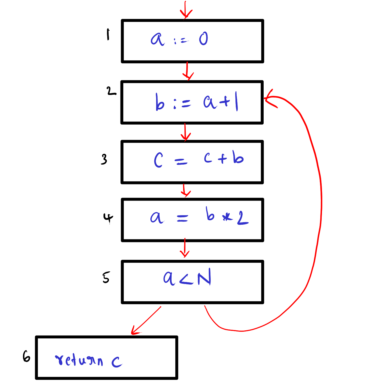
We have three temporary variables: a, b and c. Let us see where these variables are live. Note: The liveness is describe using the edges in CFG.

• a : {1->2, 4->5, 5-2}
• b : {2->3, 3->4}
• c: {1->2, 2->3, 3->4, 4->5, 5->6, 5->2}

Let us visualize this, case by case. Note: ignore the arrows in the diagram, liveness is undirected.

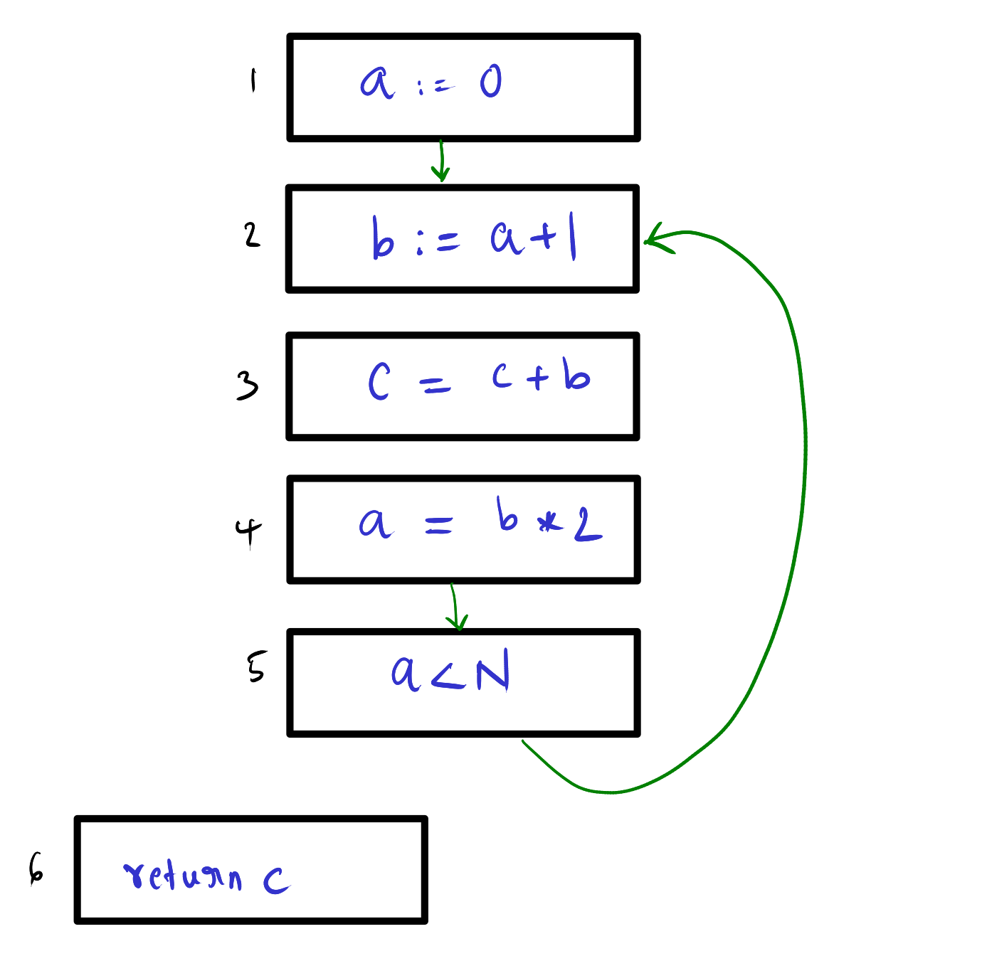
Case variable a:

The variable a is defined at 1 and then used at 2. But the usage of this definition of a ends here as you can see a is defined again at 4 (That’s why the a is not live at 2→3 and 3→4). Then a is redefined at 4 and used at 5 and 2. Hence, the liveness of a is {1->2, 4->5, 5->2}

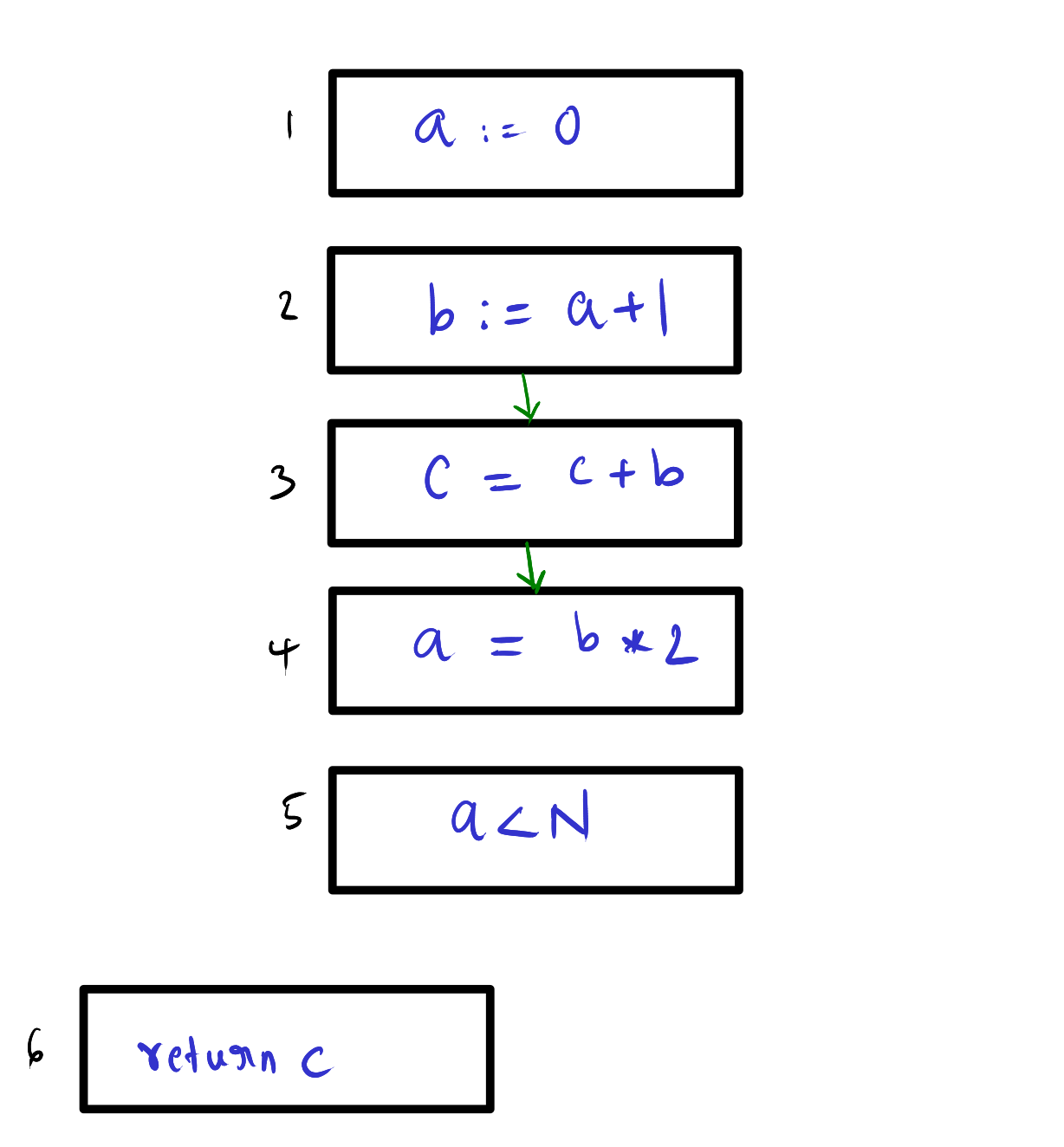
Case variable b:

This is simple, we can see the b is defined at 2 and used at 3 and 4. Hence the liveness for the b is {2->3, 3->4}.

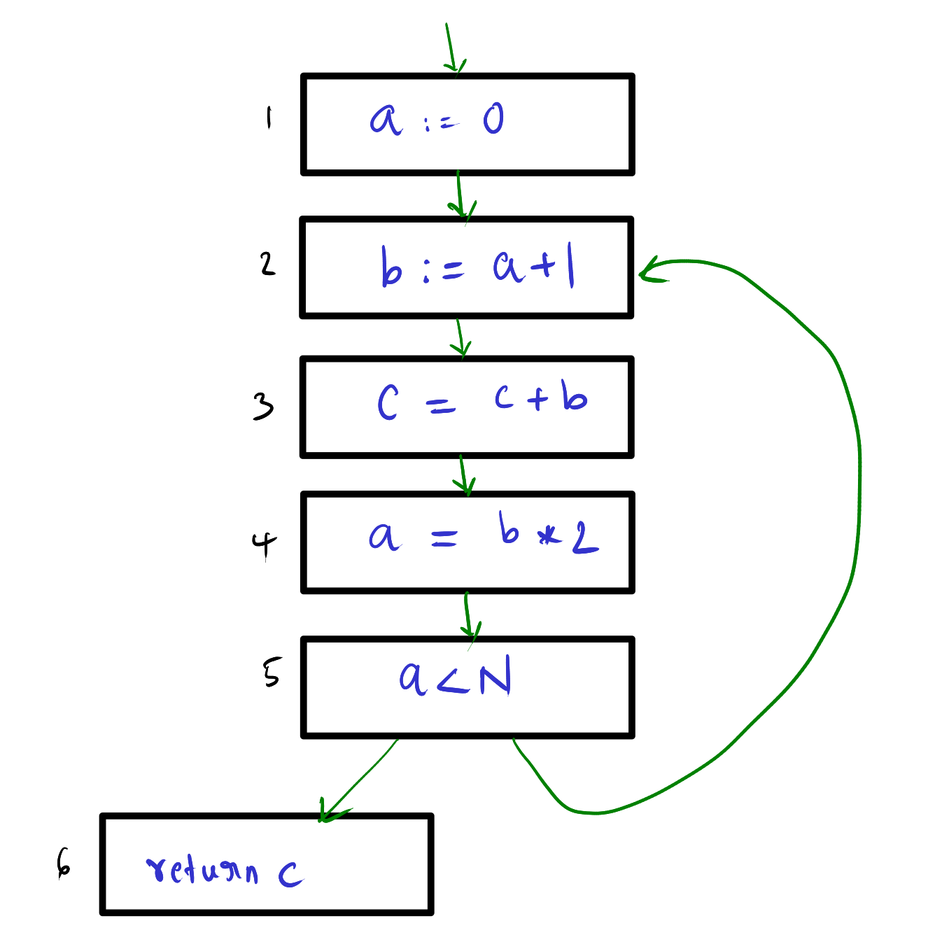
Case variable c:

We can see that c is live at the beginning of the program. And is used live inside the loop and ends at return statement, so the c is live through whole CFG in this program.

Terminology

The above problem of finding liveness of variables is an example of dataflow problem, and we say the liveness of variables flows through edges of CFG. Let us give a formal definition, which help us define dataflow equations and solving these equations provides us this liveness analysis.

Successor and Predecessor

From a node if we follow the out edges we reach all possible successors. Similarly, if we follow the in edges we reach all possible predecessors.

• succ[n] : It is the set of all successor of node n.
• pred[n] : It is the set of all predecessor of node n.

Uses and defs

An assignment statement to a variable defines that variable. An occurrence of the variable of right-hand side of statement uses that variable.

• def[n] : It is the set of variables the given node n defines.
• use[n] : It is the set of variables the given node n uses. Example: In the CFG above, for the node 3. The def[3] = {c} and uses[3] = {b, c}.

Liveness

Let us redefine the definition more formally. A variable is live on a edge if there is directed path from that edge to the use of variable without encountering a definition of that variable.

• live-in[n]: Set of variables that are live in any of the in-edges of node n.
• live-out[n]: Set of variable that are live in any of the out-edges of node n.

Calculation of Liveness

Let us define the equations which performs liveness analysis and check out the convergence of the algorithm.

Data flow equations for liveness analysis:

$$ in[n] = use[n] \cup (out[n] - def[n]) $$$$ out[n] = \bigcup_{s \in succ[n]} in[s] $$

We can describe the above equation, in three simple rules:

1. If a variable is in use[n], then it is live-in[n]. In other words, if a variable is used, then the variable is live at the point of entry.
2. If a variable is in live-in[n] then it is also live-out[] at all the nodes belonging to pred[n].
3. If a variable is in live-out[n] and not in def[n], then the variable is also in the live-in[n].

Calculation of liveness by iteration:

for each n
	in[n] <-- {};  out[n] <-- {}
repeat
	for each n
		in'[n] <-- in[n]; out'[n] <-- out[n]
		in[n] = use[n] set_union (out[n] set_sub def[n])
		out[n] = set_union(in[s]), where s is all nodes in succ[n]
until in'[n] == in[n] and out'[n] == out[n], for all n 

Convergence

The above algorithm is just applying above equations repeatedly until no changes happen to live-in and live-out. The convergence of this algorithm can be proved by monotone increase of sets and with finite number of variables in the program, we can say this algorithm converges.

Running example

Let us perform the iterative algorithm on the computation we used to defined our CFG. I am following reverse flow iteration (that is going from future to past while evaluating instruction for live-in and live-out) to reduce the number of iteration needed, but we can follow any order.

TODO: create the drawing of this table, formating is bad here

Instr	[use] [def]	out in	out in	out in
6	[c]	- c	- c	- c
5	[a]	c ca	ac ac	ac ac
4	[b] [a]	ac bc	ac bc	ac bc
3	[cb] [c]	bc bc	bc bc	bc bc
2	[a] [b]	bc ac	bc ac	bc ac
1	[-] [a]	ac c	ac c	ac c

The use and def is self-explanatory.

Let us see how the out and in for Instr 5 is defined. Others will be filled similarly Note: Before 1st iteration, all the sets are empty.

First iteration:

• First, we compute the out, we check the successor of node 5, which is {2, 6}. We add the elements in in of those two nodes. For Node 6 = {c} where as for Node 2 it is {} as we have not evaluated 2 in 1st iteration, and it was initialized with empty set. So, out[5] = {c}. Note: this follows the second dataflow equation.
• Second, we compute the in, using the first dataflow equation by doing, in[n] = use[n] set_union (out[n] set_sub def[n]). So, in[5] would be {a} + ({c} - {}) = {ac}. So, in[5] = {ac}.

We do this process on all the nodes, by iterating in this order: 6 -> 5 -> …. 2 -> 1

Second iteration:

• First, we compute out, we check successor of node 5, which is {2, 6}. We add elements in in[2] and in[6]. Note, now node 2 has been populated from first iteration. Now, out[5] = union(in[2], in[6]) = {ac} + {c}. So, out[5] = {ac}.
• Second, we compute the in, using the first dataflow equation by doing, in[n] = use[n] set_union (out[n] set_sub def[n]). So, in[5] would be {a} + ({ac} - {}) = {ac}. So, in[5] = {ac}. It remains same.

The iteration ends after 3rd as we see no changes in in and out.

How to Build an Interference Graph ?

What is a Interference Graph ?

We have large number of temporary variables, and finite number of registers. Any condition that stops allocation of same register between any two variables is called interference.

We can clearly see that we cannot assign variables to registers that are live at the same time, this is a form of interference. We will not see other possible reasons for interference, as it does not come under liveness analysis scope.

Note: For move instruction we need not add interference between variables used in the instruction, as it is kind of pointless.

Now, we see how to define interference graph. It is a graph where all the nodes denote the variables in the CFG. We define edge from x to y, if x and y have some interference.

We can generate this interference graph from liveness analysis using the following rules, which encapsulates above point:

1. Any non-move instruction that define variable a, where live-out variables are b1, b2 ... bj, then we add edges (a, b1), (a, b2) ... (a, bj).
2. At any move instruction a <-- c, where live-out variables are b1, b2, ... bj, then we add edges (a, b1), (a, b2) ... (a, bj), where bi that is not same as c.

Let us see if we can define the interference graph for above liveness analysis.

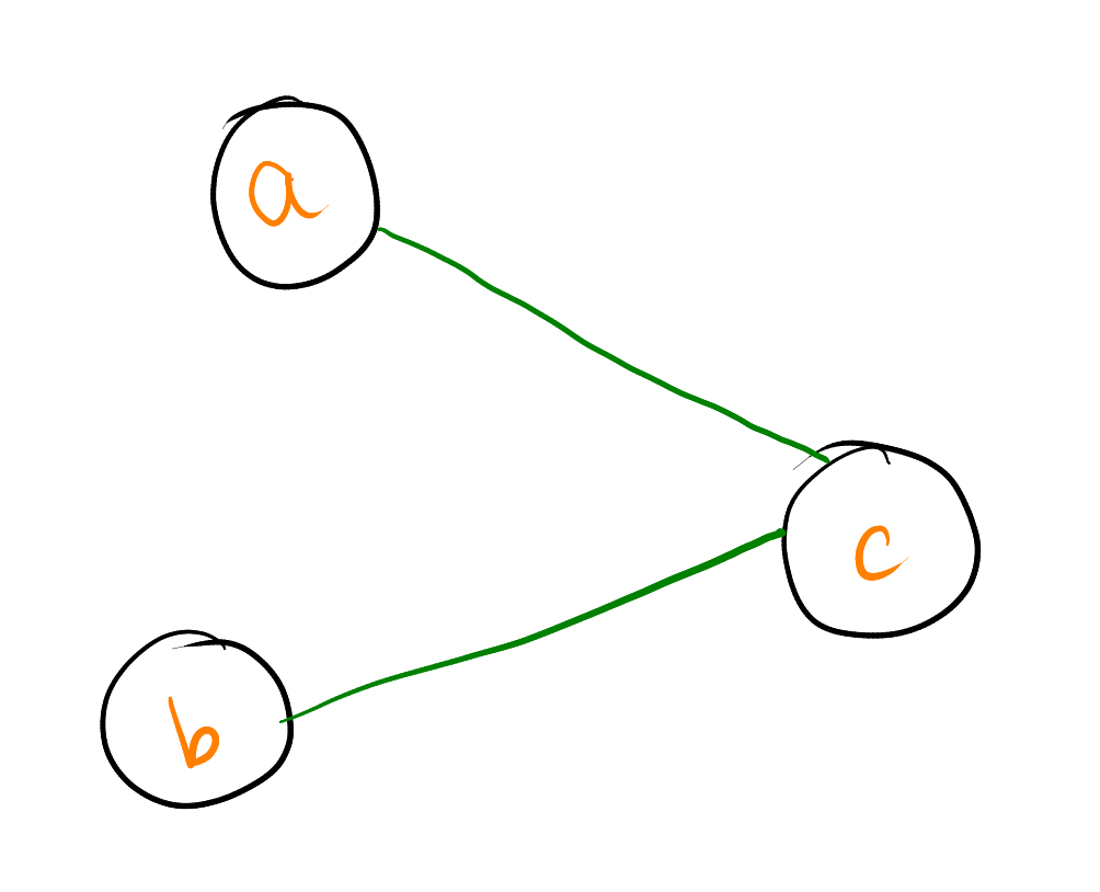
• At instruction 2, we have interference between {b} in def[2] and {c} in live-out[2]. So, we add the edges (b, c). We can get this edge in Instruction 3 as well.
• At instruction 4, we have interference between {a} in def[4] and {c} in live-out[4]. So, we add the edges (a, c).

The graph looks like this :

Coming Soon, Ocaml Implementation of the above process.

TODO….

References

• Modern Compiler Implementation in ML by Andrew Appel.